Introduction
Graph coloring is a fundamental problem in graph theory with applications in map coloring, scheduling, register allocation in compilers, and network design. The key question we explore in this tutorial is: What is the minimum number of colors needed to color a map (or network) so that no two adjacent regions (or connected nodes) share the same color?
In this tutorial, we will use metro station data from a shapefile and visualize its graph structure using Python, NetworkX, and Matplotlib. The goal is to assign colors to metro stations while ensuring that stations directly connected by a metro line have different colors.
Understanding Graph Coloring
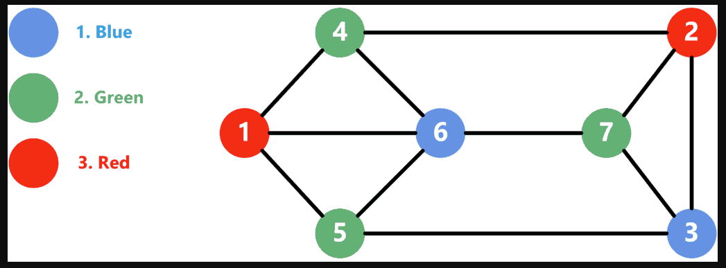
Graph coloring is an assignment of labels (colors) to the nodes of a graph such that no two adjacent nodes share the same color. The chromatic number of a graph is the minimum number of colors required to achieve this condition.
For example, in metro maps, different metro lines need to be distinguished by different colors, and adjacent stations (those directly connected by a line) should have different colors to avoid confusion.
Steps to Implement Graph Coloring for Metro Stations
We will perform the following steps:
- Load Metro Station Data: Read a shapefile containing metro station points, ensuring that each station has an identifier and a
line_numfield linking stations that belong to the same metro line. - Construct a Graph: Convert the metro station data into a graph where each station is a node, and edges exist between stations that are directly connected by a metro line.
- Apply Graph Coloring: Use a greedy algorithm to assign colors to each station while ensuring that connected stations do not share the same color.
- Visualize the Graph: Render the metro stations as a graph using NetworkX and color them based on the assigned values.
Implementation in Python
1. Install Required Libraries
Ensure you have the following Python libraries installed:
pip install geopandas networkx matplotlib shapely
2. Load Metro Station Data from Shapefile
import geopandas as gpd
import networkx as nx
import matplotlib.pyplot as plt

# Load the metro station shapefile
gdf = gpd.read_file('metro_stations.shp')
3. Create a Graph Based on Metro Lines
G = nx.Graph()

# Add stations as nodes
for idx, row in gdf.iterrows():
    G.add_node(row['station_id'], pos=(row.geometry.x, row.geometry.y), name=row['station_name'])

# Add edges for stations that belong to the same metro line
for line in gdf['line_num'].unique():
    line_stations = gdf[gdf['line_num'] == line]
    for i in range(len(line_stations) - 1):
        station1 = line_stations.iloc[i]
        station2 = line_stations.iloc[i + 1]
        G.add_edge(station1['station_id'], station2['station_id'])
4. Implement the Greedy Coloring Algorithm
def greedy_coloring(G):
    coloring = {}
    for node in G.nodes:
        # Get colors of neighboring nodes
        neighbor_colors = {coloring.get(neighbor) for neighbor in G.neighbors(node)}
        # Assign the smallest available color
        color = 0
        while color in neighbor_colors:
            color += 1
        coloring[node] = color
    return coloring

coloring = greedy_coloring(G)
5. Visualize the Graph with Colored Nodes
# Define a list of distinct colors for visualization
available_colors = ['blue', 'orange', 'green', 'red', 'purple', 'pink', 'gray', 'black', 'yellow', 'cyan']

# Assign colors to nodes based on greedy coloring
colors = [available_colors[color % len(available_colors)] for color in coloring.values()]

# Draw the graph
plt.figure(figsize=(10, 10))
pos = nx.get_node_attributes(G, 'pos')
nx.draw(G, pos, with_labels=True, node_color=colors,
        font_weight='bold', font_size=12, node_size=500, edge_color='gray', width=1)
plt.title("Metro Stations Graph Coloring")
plt.show()
Results & Insights
- The algorithm assigns colors to each metro station, ensuring that no two directly connected stations share the same color.
- The number of colors used provides an upper bound for the chromatic number of the graph.
- The visualization helps in understanding how metro networks can be effectively represented and optimized.
Optimization Considerations
- The greedy algorithm does not always guarantee the minimal chromatic number, but it is fast and works well for practical use.
- More advanced algorithms such as DSATUR or backtracking-based methods could further optimize the coloring.
Conclusion
Graph coloring is a powerful tool for solving real-world problems, including metro station visualization, scheduling, and network design. In this tutorial, we demonstrated how to construct and color a metro station network using Python, NetworkX, and Matplotlib.
By applying a greedy algorithm, we efficiently assigned colors to stations while maintaining adjacency constraints. This method can be extended to other network-based applications such as telecommunications, logistics, and clustering analysis.