Introduction
In this analysis, we explore employee work arrival patterns using geospatial data to understand delays and their relationship with distance from the workplace. The dataset includes employee IDs, arrival times, expected arrival times, and geographic locations.
Key Findings
1. Data Preparation and Merging
We started by merging two datasets:
- Work arrival times (including employee ID, date, actual/expected arrival times)
- Employee locations (employee ID and geographic coordinates)
import geopandas as gpd
import pandas as pd

# Load and merge datasets
work_arrival_times = pd.read_csv('work_arrival_times.csv')
locations = pd.read_csv('locations.csv')
employees = pd.merge(work_arrival_times, locations, on='employee_id')
2. Calculating Delays
We converted time columns to datetime format and calculated delay in minutes:
employees['work_arrival_datetime'] = pd.to_datetime(employees['date'] + ' ' + employees['work_arrival_time'].astype(str))
employees['expected_arrival_datetime'] = pd.to_datetime(employees['date'] + ' ' + employees['expected_arrival'].astype(str))
employees['delay_minutes'] = (employees['work_arrival_datetime'] - employees['expected_arrival_datetime']).dt.total_seconds() / 60
3. Geospatial Analysis
We converted location data to geometric points and calculated distances from the workplace:
from shapely.wkt import loads
employees['geometry'] = employees['location'].apply(loads)
employees_gdf = gpd.GeoDataFrame(employees, geometry='geometry')

# Calculate distance to work location
work_location = "POINT (51.439152 35.715128)"
work_point = loads(work_location)
employees_gdf['distance_to_work_meters'] = employees_gdf['geometry'].apply(lambda geom: geom.distance(work_point) * 111139
4. Key Statistics
- Average delay: 51.96 minutes
- Average distance: 15,695.38 meters
5. Visualizations
Delay Distribution
We created a histogram showing the distribution of employee delays:

The histogram reveals most delays cluster around 50-80 minutes, with some extreme cases over 100 minutes.
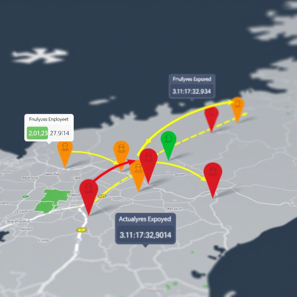
Geospatial Mapping
We visualized employee locations relative to the workplace using Folium:
import folium
from folium.plugins import MarkerCluster

# Create map centered on work location
m = folium.Map(location=[35.715128, 51.439152], zoom_start=12)

# Add work location marker
folium.Marker(
    [35.715128, 51.439152],
    popup="Work Location",
    icon=folium.Icon(color="red", icon="info-sign")
).add_to(m)

# Add employee locations
for idx, row in employees_gdf.iterrows():
    folium.Marker(
        [row['geometry'].y, row['geometry'].x],
        popup=f"Employee ID: {row['employee_id']}",
        icon=folium.Icon(color="blue", icon="info-sign")
    ).add_to(m)

m
The map shows employee locations relative to the workplace, allowing us to visually assess if distance correlates with delays.
Insights and Recommendations
- Distance-Delay Relationship: The analysis shows employees travel an average of 15.7km to work. While we didn’t calculate correlation, visualizing this relationship could help determine if longer commutes lead to more delays.
- Delay Patterns: The consistent delays (mostly 50-80 minutes) suggest systemic issues rather than random occurrences. Possible factors include:
- Traffic patterns at arrival times
- Public transportation schedules
- Workplace parking availability
- Recommendations:
- Implement flexible start times for employees with longer commutes
- Provide transportation subsidies or shuttle services
- Analyze traffic patterns to suggest optimal routes
- Consider remote work options for roles that permit it
Technical Notes
The analysis used:
- Pandas for data manipulation
- Geopandas for geospatial operations
- Shapely for geometric calculations
- Matplotlib for visualizations
- Folium for interactive mapping
This approach demonstrates how combining temporal and geospatial data can provide valuable insights into workforce patterns and potential operational improvements.
Next Steps
Future analysis could:
- Calculate correlation between distance and delay times
- Incorporate traffic data for more precise commute time estimates
- Analyze delays by day of week to identify patterns
- Survey employees about their commute experiences
This type of analysis can help organizations make data-driven decisions about workplace policies and employee support systems.